Sensor Data Logging Bandwidth Calculator
Estimate steady Mbps, burst traffic, MQTT or HTTP overhead, daily storage, and retention space for smart home sensor logging.
Run the calculator to estimate sensor logging load.
| Protocol profile | Typical added bytes | Percent allowance | Best use in this calculator |
|---|---|---|---|
| MQTT QoS 0 over TCP | About 24 B/sample | 5% | Frequent telemetry where lost single readings are acceptable. |
| MQTT QoS 1 over TLS | About 44 B/sample | 8% | Most smart home sensor streams needing delivery acknowledgement. |
| MQTT verbose topic | About 80 B/sample | 10% | Long topics, retained flags, and attribute-heavy topics. |
| HTTP keep-alive JSON | About 360 B/sample | 12% | REST sensors reusing a connection for small JSON posts. |
| HTTP new TLS request | About 900 B/sample | 18% | Polling or posting with fresh headers and connection churn. |
| WebSocket stream | About 18 B/sample | 5% | Continuous local stream with small frame headers. |
| Payload pattern | Example fields | Typical bytes | Storage behavior |
|---|---|---|---|
| Compact binary reading | ID, timestamp, value, status | 24 to 40 B | Small raw records, good compression if timestamps are delta encoded. |
| Tiny JSON state | Sensor name, value, unit | 45 to 80 B | Readable logs with moderate compression. |
| Typical JSON sensor | Topic, timestamp, value, battery | 80 to 140 B | Common home automation event record size. |
| Verbose JSON attributes | State, attributes, device class | 150 to 300 B | Attribute names repeat well in time-series storage. |
| Diagnostics batch | Multiple values and metadata | 250 to 600 B | Fewer messages but larger per-write records. |
| Scenario | Sensor count and rate | Protocol assumption | Planning note |
|---|---|---|---|
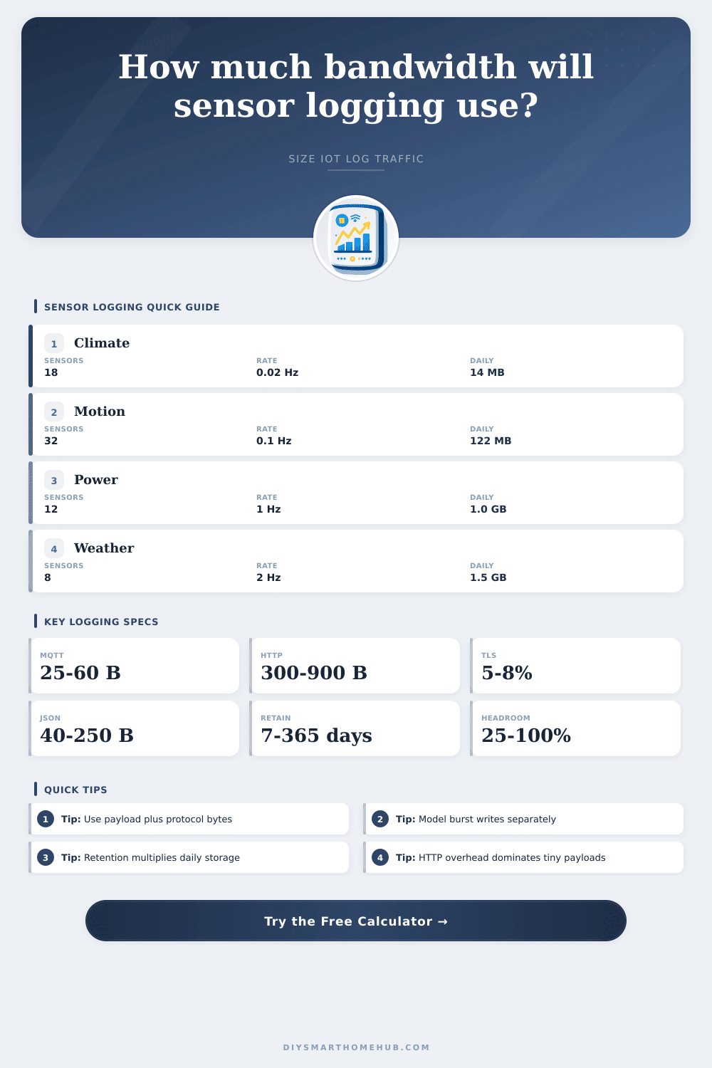
| Temperature and humidity rooms | 12 to 30 sensors, 1 per 1-5 min | MQTT QoS 0 or QoS 1 | Storage matters more than live Mbps for slow climate readings. |
| Motion and contact event logs | 20 to 60 sensors, event-based | MQTT QoS 1 | Use burst multiplier because events can cluster by room activity. |
| Power and energy meters | 4 to 24 sensors, 0.2 to 2 Hz | MQTT or WebSocket | Higher sample rates make payload size and retention visible quickly. |
| Weather and air quality | 6 to 20 channels, 0.1 to 2 Hz | MQTT verbose topic | Multiple channels per station can behave like many sensors. |
| REST polling devices | 5 to 40 devices, 5-60 sec intervals | HTTP keep-alive or new TLS | Headers can exceed the payload for very small readings. |
Five minutes, what’s that? A temperature reading every five minutes is pretty quiet, right? Well, it adds up quickly when 30 sensor start reporting in at once.” If you don’t know how much sample rate and protocol overhead grow over time, you could end up with a storage bill that rises more faster than your electricity bill instead of a neat little dashboard.
You go from peace to gigabytes of data. That’s what this load calculator does (above). It considers not only the raw sensor value but all the unseen baggage associated with each packet. That little number coming out of your wall thermostat could be tiny in size. But there is overhead: the TLS handshake required for encryption; the MQTT header telling us which device sent it; the JSON wrapper around that number carrying the data.
How to Save Space in Your Smart Home Data
This tool lets you visualize the cost of that package. How many sensors do you have? What is the size of their payload? How frequently do they report? Enter those numbers into the tool and watch as it adds on the protocol overheads, revealing actual bandwidth hit.
The cost of what you choose to send data over has been underestimated by most. When using MQTT with guaranteed delivery (QoS 1), it’s only a few dozen bytes added on each sample. Not too shabby! But then there’s HTTP. That’s another beast altogether. Payloads is nine hundred bytes if you’re polling devices and opening new HTTPS connections every time. It is fifteen times the payload of a slim MQTT solution. You’ll be able to turn those two profiles on and off in the calculator to visualize this cost-savings trade-off.
And it will show how shifting from using rest api calls to a message broker may help you save far more storage space than messing around with your compression settings ever could of. There’s also a hidden lever: sample rate. Unless you move around a lot, there’s no reason for a motion sensor to report back once a second. By dropping it down to one sample per minute, your daily data drops by a factor of six hundred. That relationship is obvious in the calculator. Adjust the samples per second, and the daily storage estimate go down. It’s forcing you to ask: do I really want that granularity? Or am I just hoarding noise?
Your daily footprint becomes a long-term liability when combined with retention policy. Logging for a month’s worth of data is doable on most home servers. A year? That typically takes serious cloud archives or dedicated hardware. Your chosen retention policy plus compression ratio equals the amount of storage required for time-series retention. Data sets like logs tend to compress very well. They cut their raw size roughly in half. However, you can’t compress infinitely. Even if you’re using extremely aggressive compression, a big daily collector fill a drive in months… Not years.
And then there’s burst traffic. And here’s the thing: Your smart home isn’t always cruising along smoothly. When a power outage occurs, suddenly all of your battery-backed sensors goes off and start alerting at once. That’s what the calculator’s burst multiplier is simulating; that traffic-storm scenario. Will it be able to get through that rush of simultaneous activity? You may have plenty of average bandwidth to cruise along just fine. However, when everybody starts talking at the same time, only a fraction of that will be available.
When you understand this variable, you stop making guesses. You begin to recognize that the number of sensors matters, but so does the choice of protocol. You understand that small payloads are killed by the right set of HTTP headers. You see that modest daily logs becomes huge annual commitments under retention policies. The numbers in the tool aren’t some abstract output. They’re a map of your infrastructure limits. Understanding where those boundaries exist makes scaling out feel less like rolling dice, it feels more like engineering. It makes your data strategy deliberate instead of reactive.
We don’t want to get rid of the data, we just want to store what’s important and avoid storing what isn’t. It’s about measuring the hidden costs of time, how often things happen, and data headers so that you can manage your own smart home memory. Store the insight and delete the baggage. The balance between the two is what makes your smart home truly smart.