Sensor Data Logging Storage Calculator
Estimate storage for smart home sensor telemetry using payload size, sample rate, sensor count, retention days, encoding overhead, compression, duty cycle, and upload bandwidth.
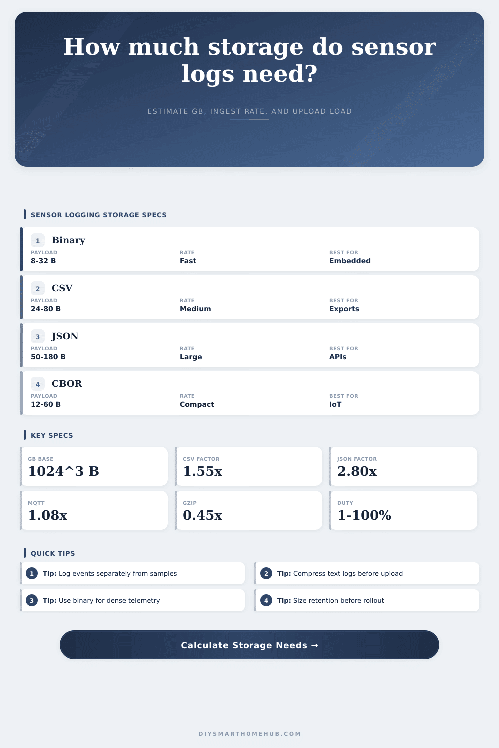
Best for dense numerical telemetry, embedded logs, and gateways that do not need human-readable rows.
Useful for spreadsheet exports, but repeated delimiters and timestamps add predictable storage overhead.
Convenient for APIs and debugging because field names travel with each sample, but it expands small readings.
Works well on repetitive text logs, stable timestamps, repeated sensor ids, and slow-changing measurements.
| Encoding | Multiplier | Typical record shape | Storage note |
|---|---|---|---|
| Binary or packed protobuf | 1.00x | Timestamp, id, value bytes | Use when dashboards can decode compact records. |
| CBOR or MessagePack | 1.20x | Compact typed fields | Good middle ground for gateways and local databases. |
| CSV with timestamp | 1.55x | Delimited row text | Readable and exportable, but timestamps repeat on every row. |
| JSON per sample | 2.80x | Named object text | Field names, quotes, and punctuation dominate small sensor records. |
| Time-series blocks | 1.35x | Chunk plus tags | Often balanced when retention queries matter. |
| SQLite row storage | 1.85x | Rows plus indexes | Indexes speed lookup but add database overhead. |
| Protocol source | Overhead factor | Included metadata | Planning use |
|---|---|---|---|
| Stored locally only | 1.00x | No extra transport envelope | Use for final database size when messages are parsed before storage. |
| MQTT telemetry | 1.08x | Topic, QoS, small packet fields | Good for retained queue or broker-side archive sizing. |
| HTTP webhook batch | 1.18x | Headers amortized over a small batch | Use for gateway upload queues and simple cloud ingestion logs. |
| Matter or Thread bridge | 1.12x | Bridge source and cluster metadata | Useful when normalized hub events preserve device model context. |
| Zigbee gateway metadata | 1.10x | Endpoint, cluster, link quality | Use when raw gateway exports keep radio diagnostics. |
| Bluetooth LE gateway | 1.06x | Gateway id and RSSI fields | Often compact unless scan packets are stored raw. |
| Sensor log type | Raw bytes/sample | Common rate | Duty cycle note |
|---|---|---|---|
| Temperature and humidity | 24 to 40 B | 1 every 1 to 10 min | Usually continuous but slow-changing. |
| Door or window contact | 28 to 70 B | Events plus heartbeat | Often 1% to 10% active logging duty. |
| Water leak sensor | 32 to 80 B | Heartbeat plus alerts | Low event count, long retention is easy. |
| Energy or power meter | 36 to 96 B | 1 every 5 sec to 1 min | Continuous samples can dominate a home database. |
| Air quality monitor | 80 to 220 B | 1 every 10 sec to 5 min | Many fields per sample increase bytes before encoding. |
| Motion or occupancy | 32 to 120 B | Events plus state | Burst logging may matter more than average rate. |
| Reference workload | Example inputs | Approx daily data | Separate planning note |
|---|---|---|---|
| Small sensor set | 12 sensors, 32 B, 0.2/min, CSV | About 1 MB/day | Long retention usually fits on small local storage. |
| Whole-home telemetry | 60 sensors, 64 B, 1/min, JSON | About 15 MB/day | Compression and downsampling matter over multiple years. |
| Fast power meter group | 10 sensors, 80 B, 12/min, binary | About 8 MB/day | Sample rate dominates even with compact encoding. |
| One 1080p camera | 2 Mbps continuous video | About 21 GB/day | Camera video storage is separate from sensor sample math. |
Getting to see real-time data pouring in from temperature sensors is exciting, until you realize your hard drive fills up and panic ensues. Because disk space are a physical limit, it must be planned for before receiving any bytes. And most folks just begin with hardware and assume the software will take care of things after-the-fact, only to find themselves with lost history and empty space.
The result depend on a handful of initial math decisions. How many details? Ultimately, this is your decision: How much do you really care about? An air quality monitor that logs 10 times per second produce a lot of data; a climate sensor that logs every five minutes produces relatively little. Once you know the rate at which each sensor will sample and how many sensors you’ll use, the math are done for you by the calculator above (so you don’t have to guess).
How to Plan Your Sensor Data Storage
The number of samples per minute matter more than the total number of minutes. Do you need to capture every tiny change in your environment? Or are you happy with just an hourly average to detect leaks? While high-rate sampling sounds thorough, it can absorbs nothing but noise. If your environment doesn’t change much (e.g., soil moisture), you’re wasting your own bandwidth (i.e., paying for storage) and aren’t benefiting from high rates.
However, that doesn’t mean that we should stick with these formats regardless, because the answer also depends heavily on how you plan to read them. While machines love binary formats (they are compact and efficient), people hate reading broken valves at 2AM from a binary file. While JSON is flexible and readable by humans, it has a big tax due to repeating field names at every sample. If you’re logging a thousand doors, that’s going to quickly add up, meaning JSON could need twice or even three times as much storage than a binary format.
CSV falls somewhere in between: it still repeats timestamps, which is good for exports but bad for other uses. As seen on the page, this means a 30-byte binary record balloons to almost 90 bytes in JSON. A three times increase just to make your human eyes happy.
That’s where compression comes into play. It is another great equalizer. Compression algorithms like gzip and others finds patterns in repetitive strings of characters (they do this best with text). So if all your field names and sensor IDs is the same, then they’ll compress down nicely. But remember that compression use CPU cycles. While a beefy gateway server will be able to compress data before uploading without any problem, a humble little battery-powered node may not.
Again: there are no free solutions. Only tradeoffs. Do you want to compress files in the cloud? You’ll save on battery life but pay extra for data uploads. Do you want to compress on the edge? You’ll save bandwidth, but burn more batteries.
The other lever that most people ignore till it’s too late is called duty cycle. All sensors aren’t always talking. A water leak sensor may only send a heartbeat once an hour while a door contact may sit silent for days. Setting the duty cycle to 100 percent for an event-driven sensor will wildly overestimate your needs. Setting a duty cycle of 100 percent for a power meter will wildly underestimate your needs. Think about how often the thing being measured change. Does it sit still? Or does it change constantly?
And that’s when you see the price tag: retention policy. Do you really want to keep every piece of data forever? No. Generally, most systems requires high-resolution data for a limited period of time and then downsampling aggregations over a longer period. Why would you want second by second temperatures for last Christmas? You don’t. You want the daily average.
If you plan accordingly for this type of layered system, both your storage footprint will be reasonable and your queries will remain fast. Don’t store all of it. Store just enough. Store enough to answer questions like “did the basement flood on Tuesday?”
You shouldn’t of need a server farm to do this; just start by getting the basics. Go as coarse a sample rate as possible while still telling the story. Encode using a format that strikes a balance between size and readability. Compress where appropriate. Check the numbers. How does that look? Does the amount of data taken in each day fit your bandwidth? Great! Dial back if needed.
Losing some precision is preferable to losing the ability to have access to the data. Storage is cheap. Space isn’t. Plan for the end from the beginning.