Fiber Optic Distance Calculator
Estimate maximum fiber link distance from transmitter power, receiver sensitivity, fiber attenuation, connectors, splices, safety margin, and modal bandwidth limits for home lab, camera, AP, and backbone runs.
📌Fiber link presets
⚙Optical link inputs
Fiber Link Result
Optical budget and modal bandwidth are checked together.
Formula Breakdown
📊Selected fiber and transceiver spec grid
Short-reach multimode optics.
Typical 850 nm multimode attenuation.
OM3 effective modal bandwidth.
TX power minus receiver sensitivity.
📝Fiber attenuation reference
| Fiber profile | Wavelength | Typical attenuation | Planning use |
|---|---|---|---|
| OM2 multimode | 850 nm | 3.5 dB/km | Legacy short 1G or limited 10G links. |
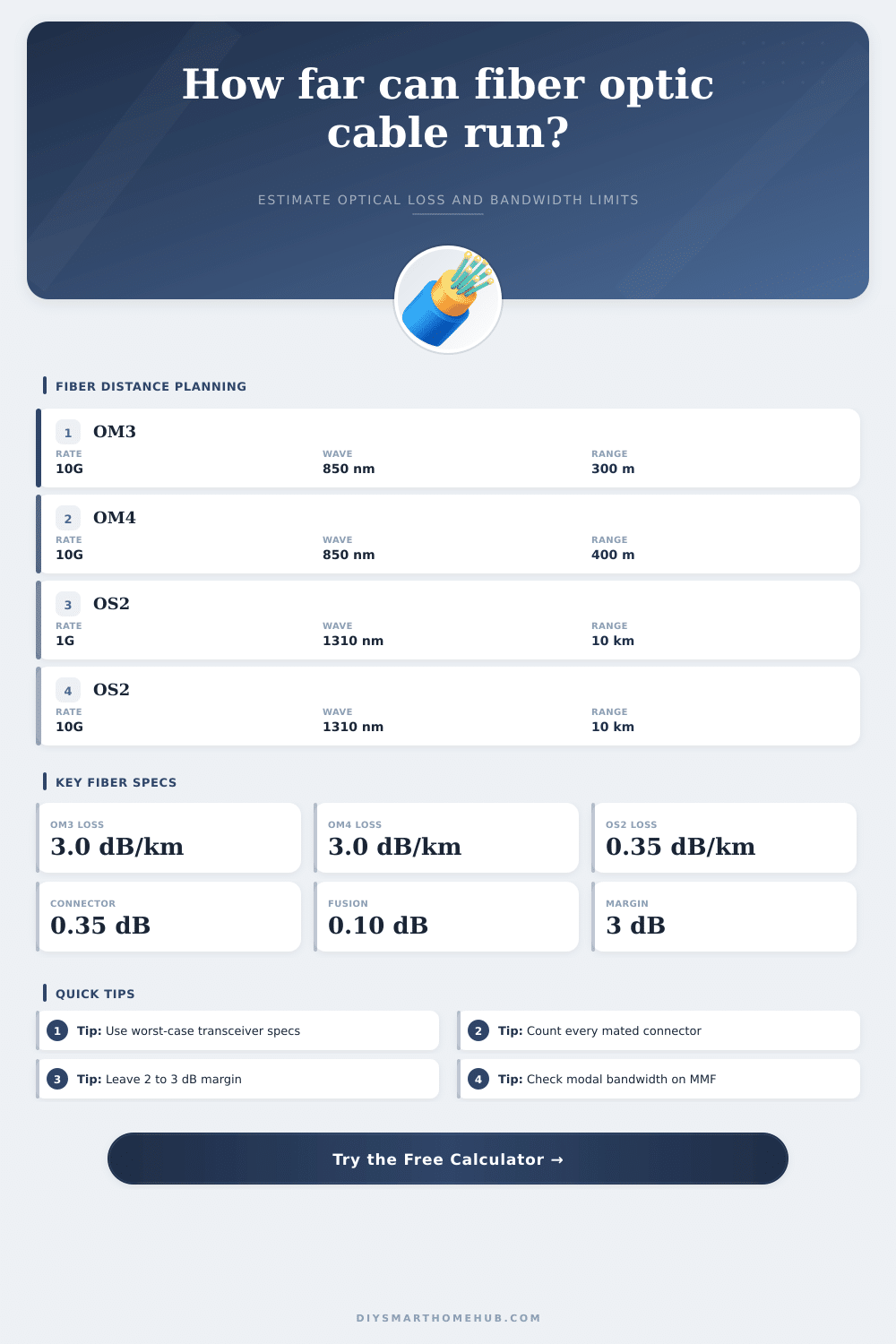
| OM3 multimode | 850 nm | 3.0 dB/km | Common 10G SR runs to about 300 m when bandwidth allows. |
| OM4 multimode | 850 nm | 3.0 dB/km | Higher modal bandwidth for longer 10G SR channels. |
| OS2 single-mode | 1310 nm | 0.35 dB/km | Campus, outbuilding, and long backbone optics. |
| OS2 single-mode | 1550 nm | 0.22 dB/km | Longer reach optics where equipment supports 1550 nm. |
🔎Transceiver optical budget table
| Optic class | Typical TX used | Receiver sensitivity | Calculator note |
|---|---|---|---|
| 1000BASE-SX | -4.0 dBm | -17.0 dBm | Large loss budget, but multimode bandwidth controls distance. |
| 1000BASE-LX | -3.0 dBm | -19.0 dBm | Often used with OS2 for 5 km to 10 km class links. |
| 10GBASE-SR | -1.0 dBm | -11.1 dBm | Short-reach multimode, usually bandwidth-limited. |
| 10GBASE-LR | 0.5 dBm | -14.4 dBm | Single-mode link budget supports 10 km class runs. |
| 40G/100G SR4 | -2.0 dBm | -9.0 dBm | Parallel multimode optics need the shortest bandwidth check. |
🔢Formula reference table
| Step | Formula | What it checks | Result card |
|---|---|---|---|
| Optical budget | TX power - receiver sensitivity | Total dB available before losses. | Power budget left |
| Fixed losses | Connector loss + splice loss + safety margin | Loss not caused by cable distance. | Planned link loss |
| Fiber loss | Distance km x attenuation dB/km | Cable attenuation along the route. | Planned link loss |
| Max loss distance | (Budget - fixed losses) / dB per km | Longest optical-power-limited link. | Max distance |
| Modal bandwidth | Bandwidth MHz km / data rate MHz | Multimode dispersion distance estimate. | Bandwidth limit |
🏠Common fiber run examples
| Scenario | Typical fiber | Distance cue | Main limiting factor |
|---|---|---|---|
| Same rack DAC replacement | OM3 or OM4 | 5 m to 30 m | Connector count and optic type. |
| Room to network closet | OM3 10G SR | 50 m to 150 m | Usually modal bandwidth reserve. |
| House to detached garage | OS2 1G LX | 100 m to 500 m | Mostly connector and splice losses. |
| Gate or camera pole | OS2 10G LR | 300 m to 2 km | Optical budget with outdoor splices. |
| Small campus backbone | OS2 10G LR | 1 km to 10 km | Transceiver budget and margin. |
💡Fiber distance tips
Have you ever been so close, just a meter too short, of the switch only to yank another cable and see the link light flicker madly but eventualy go dark? It’s happened to me more times than I can count, particulary where a mix of transceivers and fiber types is involved. The calculator above check for two different failure modes so that you won’t pull a single wire by mistake.
Optical power is what most folks think about, “if it makes it there, the signal will get through.” In multimode, however, modal bandwidth frequentlly murders a link well before attenuation do. First, let’s differentiate dispersion limit vs. Loss budget. Dispersion limit’s pretty simple: it’s the maximum distance that pulses can travel before they spread out and overlap (causing bit errors). That’s why “mode”, how different light paths travel at slightly different speeds down the strand; matter; if those pulses smear together, your max distance gets very small real fast.
How to Choose Fiber Optic Cable and Transceivers
Loss budget is just plain math based off the power output of the transmitter, the sensitivity of the receiver, and the losses across connectors/splices/etc. Luckily, the tool take all this into account and saves us from fumbling with dBs. All you do is specify your hardware, plug in your intended distance, then add number of connector pairs you intend to mate. Believe it or not, that’s actualy a major source of loss on a short run. A typical LC pair will increase your overall loss by about 0.35 dB, so four will use 1.4 dB before the photons has even reached their fiber glass home.
The problem is dispersion. Intuition won’t get us far here; in multimode fiber (like OM3 or OM4), there are multiple light mode traveling down the fiber at slightly different speeds. If you run them fast enough, they will disperse. They will overlap one another and produce bit errors. These error appear as random noise instead of just a loss of signal. This is why the calculator divide the modal bandwidth by your data rate to calculate a hard distance limit. You might have ten decibels of remaining power, but you can only push 10 Gigabit Ethernet about three hundred meters through OM3 fiber before the pulses smear into each other. And that is what everyone miss when upgrading their office backbone.
Choosing between single-mode and multimode depends on your distance requirements, existing infrastructure, and the technical limits of dispersion and power budgets. If you have existing multimode in place, clearly use it. And if you want something that will run further than four hundred meters, single mode is a must as it uses a small fiber core that funnels light down one narrow path removing virtually all modal dispersion. Standard LR transceivers allows runs of up to ten kilometers. Even better, its low attenuation is typically less than half a decibel (0.35) per kilometer at 1310 nanometers. This means you can pull pretty far before running out of power budget.
No spreadsheet will perfectly anticipate what happens with real-world installation. The connectors aren’t as well polished as assumed, which introduce more than the typical 0.35 dB of scattering losses. Bending the fiber too sharply around a corner causes macrobending loss, which deplete signal strength in unexpected ways. And it’s always a good idea to include a three-decibel margin in your design for imperfect splices, component aging, and the expected temperature fluctuations. That buffer keep the link stable several year post-installation when equipment degrades ever so slightly and dust builds up inside.
For example, before planning a new run, decide what speed or data rate will be needed for it and how far it needs to go. Do you have single-mode cable available already in your conduit? Or do you have to pull some? Are you stuck using older OM2 or OM3 infrastructure? Will those transceivers you’re looking at actualy work at that speed across that kind of glass? The page has a couple of handy reference tables that outline the usual transceiver budgets and attenuation values. These can serve as guidelines for making this call, so there is no need to get your physics degree out.
All in all, designing for success boils down to understanding bandwidth limitations and adhering to power limits. Without one, you would of been getting midnight calls trying to troubleshoot something that shouldn’t have been built in the first place. With each meter of multimode fiber being viewed as an opportunity for dispersion and each connector as a possible leak, you are building something that works right out of the box. It’s a solid link that endures over time through environmental shifts and equipment upgrades. Some forethought goes a long way to avoid the blinking light hell later.