Fiber Optic Splitter Loss Calculator
Estimate equal split or tap splitter loss, excess loss, wavelength fiber attenuation, connector and splice loss, received power, and usable link margin.
📌Splitter network presets
⚙Optical path inputs
Fiber splitter result
Run the calculator to see the link budget.
💡Splitter and fiber spec grid
The ideal loss of an equal splitter rises with the number of output branches.
An unequal splitter uses the selected output percentage for branch-specific loss.
Single-mode fiber attenuation changes by wavelength and cable condition.
Leave headroom for repairs, aging, patch changes, and real splitter variance.
📋Reference tables
| Splitter | Theoretical loss | Typical PLC loss | Planning note |
|---|---|---|---|
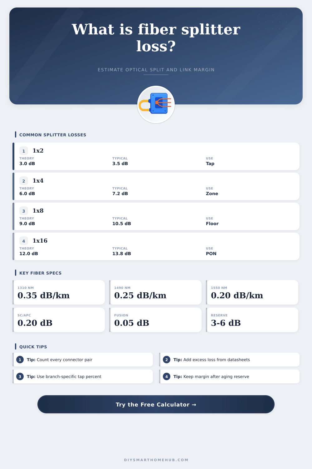
| 1x2 equal | 3.01 dB | 3.4 to 3.8 dB | Small tap, lab feed, or redundant path. |
| 1x4 equal | 6.02 dB | 6.8 to 7.4 dB | Compact cabinet or small distribution zone. |
| 1x8 equal | 9.03 dB | 10.0 to 10.8 dB | Floor, small MDU, or long hallway branch. |
| 1x16 equal | 12.04 dB | 13.2 to 14.2 dB | Common passive optical network branch count. |
| 1x32 equal | 15.05 dB | 16.5 to 17.8 dB | High split needs strong budget discipline. |
| 1x64 equal | 18.06 dB | 20.0 to 21.5 dB | Usually needs short fibers or high-class optics. |
| Wavelength | Typical SMF loss | Common role | Calculator use |
|---|---|---|---|
| 1310 nm | 0.35 dB/km | Upstream and short reach optics | Use for upstream loss checks. |
| 1490 nm | 0.25 dB/km | PON downstream data | Good default for home fiber drops. |
| 1550 nm | 0.20 dB/km | Video overlay and long reach | Lowest normal attenuation band. |
| 1625 nm | 0.24 dB/km | Monitoring and test channels | Useful for maintenance wavelength checks. |
| Component | Conservative loss | Good loss | Counting rule |
|---|---|---|---|
| SC/APC connector pair | 0.30 dB | 0.15 to 0.20 dB | Count each mated adapter pair. |
| LC/UPC connector pair | 0.40 dB | 0.20 to 0.30 dB | Use higher value for mixed patching. |
| Fusion splice | 0.10 dB | 0.02 to 0.05 dB | Count each permanent splice. |
| Mechanical splice | 0.20 dB | 0.10 to 0.15 dB | Use for field repair or temporary joints. |
| Network preset | Split model | Typical length | Margin cue |
|---|---|---|---|
| ONT Closet 1x2 | Equal 1x2 | 0.08 km | Usually easy when patch loss is controlled. |
| Rack 1x4 Lab | Equal 1x4 | 0.15 km | Watch connector count more than fiber length. |
| Floor 1x8 | Equal 1x8 | 0.55 km | Moderate split with several patch points. |
| PON 1x32 | Equal 1x32 | 2.8 km | Needs clean splices and measured splitter loss. |
| 90/10 Tap | Tap branch | 0.35 km | The 10 percent branch takes the larger hit. |
🔧Practical planning tips
The fiber optic power meter reads something that is just barely green. That’s a moment of concern. Now it’s not some hypothetical exercise.
The signal has to get from here (you’re in an air-conditioned equipment room) to there, with all those connectors and bends and splits along the way. And it has to do so while passing through a material (glass) different than air. The light has to be bright enough when it reaches the receiving end to make a difference.
How to Calculate Light Loss in Fiber Optics
Loss is additive, and getting it right require knowing that it adds up. But you also need to know that adding up doesn’t feel like linear addition. It feels exponential, which is why we have logarithms. After plugging in your topology, the calculator above do all the math for you. You no longer have to go through the hassle of converting back and forth between decibels and linear ratio each time you add an additional connector.
What’s the worst thing most people do? They only consider the splitter itself. Yeah, so a 1 x 8 split doesn’t sound like much, until you remember that the optimal splitting loss alone use nine decibels. That’s nearly half your budget consumed before the light ever reaches a single meter of fiber. Then you need to factor in excess loss as well. Excess loss refers to flaws within PLC chip (or planar lightwave circuit). It’s tiny, typically one decibel, but it adds up and it exists.
The thing is that glass absorbs wavelengths of light different depending on their color. So 1310 nanometers, which we use for our upstream data, has more signal loss per kilometer then 1490 nanometers, which we use for our downstream traffic. Pick the wrong one and you will have more loss. That’s explained well in the reference table found on the page. You’ll notice that even a little bit of fiber add up quickly when you choose the incorrect wavelength band for the distance. In fact, most passive optical networks runs specific wavelengths to ensure downstream traffic doesn’t interfere with upstream traffic. Match your loss calculation to your actual signal path.
The other place where budgets quietly bleed out is at connectors. A patch panel is a pass-through right? Wrong. Each mated connector pair contribute some insertion loss and back reflection. Back reflection can be minimized with an APC (angled physical contact) connector which angles the ferrule to prevent light bouncing back into the source laser. This happens for a specific reason. Twenty pairs of connectors in your link budget? Even a modest half-decibel loss per pair will adds up to ten decibels total, the difference between a stable connection and one that flickers when it’s loaded.
The quality of the installation is another tale told by splices. In general, fusion splices is cleaner than mechanical ones. Done right, they add virtually no measurable loss. However, when planning, don’t ignore them. Those little losses don’t go away because they’re little; you have to add them all together on a long run with lots of joints. You’ll be able to plug in those variables separately and see exactly what the bottlenecks realy are.
The safety net is called link margin. You should of never design a system that operates exactly at the edge of the receiver’s sensitivity. Plan for aging; plan for dirt on connectors; plan for having to repatch something later. After allowing for both aging and reserves, if you have no positive margin left over then your links won’t survive in real world. Better to find out now rather than when it’s down for service.
These elements turn designing fibers from guesswork into engineering. You no longer view loss in terms of some vague figure; instead, you visualize tangible obstacles that light beam must overcome. And you realize it’s not about moving light from Point A to Point B. It’s about delivering it with enough strength so it can transport your data dependabelly for years. Respect the decibels, and your link will stand firm.